On-Demand Spectrograms via GPU Compute

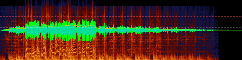
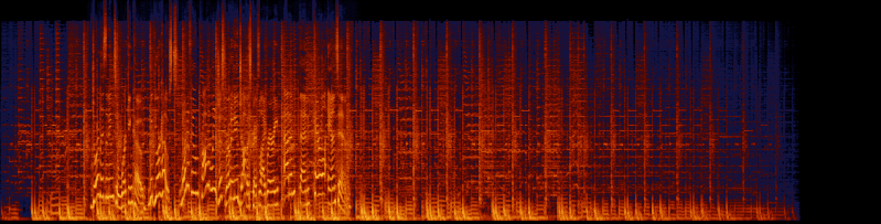
I'm building Engineering, an offline audio processing workstation in the vein of iZotope RX. Users import audio, build processing graphs (denoise, de-click, isolate dialogue, rebalance stems), and inspect results on a timeline. Waveforms and spectrograms are essential to that workflow. The core visualization problem: how do you turn raw PCM samples into a spectrogram and waveform display without making the user wait?

The naive approach is to pre-compute everything at import time. Run an FFT over the entire file, write the frequency magnitudes to a binary file on disk, and load byte ranges into memory when the user scrolls or zooms. This means processing every sample in the file upfront, which takes minutes for long recordings. It also means maintaining binary formats, IPC for range reads, a dual-layer loading system, and a separate rendering pipeline. Changing any analysis parameter (FFT size, frequency scale) means re-processing the entire file.

The insight that changed everything was twofold. First, you don't need to compute the spectrogram for the entire file. You only need the samples that are currently visible, at pixel resolution. Second, WebGPU compute shaders are available in the browser, giving you GPU parallel compute that you can't access from Node.js. Each FFT window runs as an independent workgroup, so thousands of them process in parallel. Two compute dispatches produce a final RGBA texture from PCM input. No binary files on disk, no loading pipeline. Settings changes recompute instantly. Load times dropped from minutes to seconds.

The CPU side handles what doesn't parallelize: waveform min/max, loudness metering (BS.1770-4), RMS, peak, and true peak. All computed in a single streaming pass alongside the GPU work.

I assumed spectrograms were too expensive to compute on the fly. That assumption led to a caching system that was more complex than the computation itself. It turns out that when you can dispatch thousands of FFT windows in parallel, "just compute it when you need it" is both faster and simpler than maintaining a pre-computed cache.

Published as @e9g/spectral-display.